Shortcuts in Fisher Exact P-values, part 1

I’ve been reading up on Fisher exact p-values (FEP)

Books

• “CIforSSBS”: Causal Inference for Statistical, Social, and Biomedical Science, by Guido W. Imbens and Donald B. Rubin, chapters 4-5 (it helped a lot to read this first)
• “Mixtape”: Causal Inference: The Mixtape, by Scott Cunningham, section 4.2
• “1stCourse”: A First Course in Causal Inference, by Peng Ding, chapter 3 (see here)

Papers

• “Bind & Rubin”: “When possible, report a Fisher-exact P value and display its underlying null randomization distribution”, by M.-A.C. Bind and D.B. Rubin (cited in 1stCourse)
• “Thornton”: “The demand for and impact of learning HIV status: Evidence from a field experiment”, by Rebecca Thornton (cited in Mixtape)
• “Pashley et al”: “Conditional As-If Analyses in Randomized Experiments”, by Nicole E. Pashley, Guillaume W. Basse, Luke W. Miratrix

A couple things I want to do

• Discuss shortcuts/substitutions in Mixtape and 1stCourse, why they’re ok, but one shortcut has drawbacks in general
• Make plots of the Fisher null distribution for Mixtape

1. Shortcuts/substitutions used

Mixtape makes three shortcuts

1. Analyzes a Bernoulli trial as a completely randomized experiment (CRE)
2. Samples from the set of all permutations of the assignment vector
3. Samples with replacement

1stCourse makes shortcuts 2 and 3. I tried to determine if it also made shortcut 1, because I couldn’t immediately find how the data randomization was done, and I decided to not spend too much time digging.

2. Analyzing a Bernoulli trial as if completely randomized

In section 4.6, Mixtape estimates Fisher exact p-values for data from Thornton, as if it were completely randomized. Thornton describes the randomization process:

Voucher amounts were randomized by letting each respondent draw a token indicating a monetary amount out of a bag… If a respondent drew a token indicating zero incentive, no voucher was given to the respondent; 20 percent received no incentive

Then, using positive incentive as treatment, it was a Bernoulli trial with $p(W_i = 1) = 0.8$ (ignoring some irregularity described in the paper).

Is it ok to analyze a Bernoulli trial as if it were completely randomized? It’s not immediately clear that it should be.

Pashley et al:

The injunction to ‘analyze the way you randomize’ is well-known to statisticians since Fisher advocated for randomization as the basis of inference.

Bind and Rubin:

The Fisherian statistical framework, proposed in 1925, calculates a P value in a randomized experiment by using the actual randomization procedure that led to the observed data.

(Emphasis added to both.) These quotes would point to the data needing to be analyzed as a Bernoulli trial.

However, both papers also justify analyzing data differently, in some cases. In particular, they both support analyzing a Bernoulli trial as if it were completely randomized.

Bind and Rubin:

Of course, we advise knowing the actual assignment mechanism, but not necessarily following it to conduct randomization-based inference; the reason is that many statisticians recommend conditioning on ancillary statistics

Pashley et al create a technical notion of validity, show that Bernoulli-as-if-completely-randomized is valid, and discusses the benefits of analyzing this way

why should we consider alternative as-if analyses, even valid ones? … A natural, but only partially correct, answer would be that the goal of an as-if analysis is to increase the precision… [however] The primary goal of an as-if analysis is not to increase the precision of the analysis but to increase its relevance.

and later,

Our theory suggests that one can, and in fact should, analyze an experiment in a way that is both compatible with the original randomization and also relevant to the observed data.

3. Using permutations of the assignment vector

For a completely randomized experiment, let $n_\text{treat}$ be the number of treated, $n_\text{ctrl}$ the number of controls, and $n_\text{total} = n_\text{treat} + n_\text{ctrl}$. With data indices $0, 1, \ldots, n_\text{total} - 1$, the set of allowed assignment vectors is equivalent to the set of all combinations that select $n_\text{treat}$ indices, and there are $N_\text{comb} := \binom{n_\text{total}}{n_\text{treat}} = \frac{n_\text{total}!}{n_\text{treat}!n_\text{ctrl}!}$

such combinations.

Earlier examples in Mixtape and 1stCourse have smaller datasets, and those examples use the full set of completely randomized assignment vectors (Mixtape sections 4.2.1 and 4.2.4, 1stCourse section 3.2). The books each present an example with a larger dataset, where $N_\text{comb}$ is prohibitively large, they make their inference using a sample of the assignment vectors (Mixtape 4.4, 1stCourse 3.4). Both draw their samples by permuting the assignment vector.

Take a fixed assignment vector, with $n_\text{treat}$ 1’s and $n_\text{ctrl}$ 0’s. There are $n_\text{treat} ! n_\text{ctrl}!$ ways to permute the vector indices without changing the assignment (permute within the 1’s and within the 0’s without permuting between the 1’s and 0’s). The effect of using permutations is that the sampling of assignment vectors is done with replacement.

How important is it that the sampling is done with replacement?

4. Sampling with replacement

To understand the effect of sampling with replacement, I’ll use the same examples as in Mixtape and 1stCourse, and one outcome from Bind & Rubin. I’ll sample with replacement (i.e., sampling from permutations) and without replacement (i.e., ensuring sampled assignment vectors are unique), and compare.

Long story short: When the number of samples $k$ is tiny relative to the number of possible assignment vectors (i.e., when $k / N_\text{comb}$ is small), there’s basically no difference, because there will be few or no duplicate draws. When $k / N_\text{comb}$ is larger, duplications will increase, and the main impact will be increased variance of FEP estimates.

4.1 Mixtape

The data is available from Mixtape’s GitHub repo in thornton_hiv.dta.

For this data $N_\text{comb} = \binom{2901}{2222}$, and Mixtape used three simulations with $k$ equal to 100, 500, and 1000 samples. With these numbers, the probability of any duplicates is effectively zero.

Mixtape used ATE as test statistic. The sampled null randomization distributions (i.e, the distribution of ATE for sampled assignment vectors) are very similar, and the p-value estimates are identical (< 0.001). As they should be, since there is almost no chance of duplicate draws. The plots below are for $k = 1{, }000$.

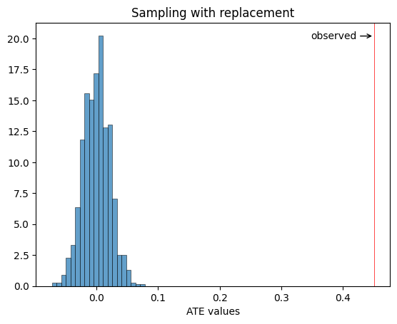
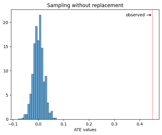
It’s striking how far the true ATE value is from the sampled null distribution. As Mixtape says

We could throw atom bombs at this result and it won’t go anywhere.

The strength of the results is demonstrated by the p-value, but it somehow feels even more extreme on the plot. As Bind & Rubin says

we may learn something scientifically interesting from examining the shape of the null randomization distribution

4.2 1stCourse

The data is available here, “NSW Data Files (Dehejia-Wahha Sample)”.

For this data $N_\text{comb} = \binom{445}{185}$, and 1stCourse used $k = 10{, }000$ samples. The probability of any duplicate draws is again effectively zero, meaning the null randomization distributions and p-values should be very similar. I double-checked this using the t-test with unequal variance and got similar plots and identical p-value estimates. 1stCourse has plots of the null randomization distribution; no need to replicate them here.

4.3 Bind & Rubin

Bind & Rubin calculated Fisher exact p-values for 484,531 outcomes, each with $N_\text{comb} = \binom{17}{10} = 19{, }448$ possible assignment vectors. They describe the massive amount of computation required (they used an high-performance computing cluster), and suggested the possibility of reducing compute by sampling the assigment vectors.

Suppose a researcher wanted to reduce the compute burden by sampling $k = N_\text{comb} / 4 = 4{, }862$ assignment vectors for each outcome.

With $k = N_\text{comb} / 4$ or $k / N_\text{comb} = 1 / 4$, it is almost a certainty that there will be duplicates. In fact, we can expect roughly 12% of draws will duplicate a previous draw. However, the null randomization distribution are still very similar (I expected more difference). Here are the distributions for outcome D, using just the first period of the experiment (see the paper for details).

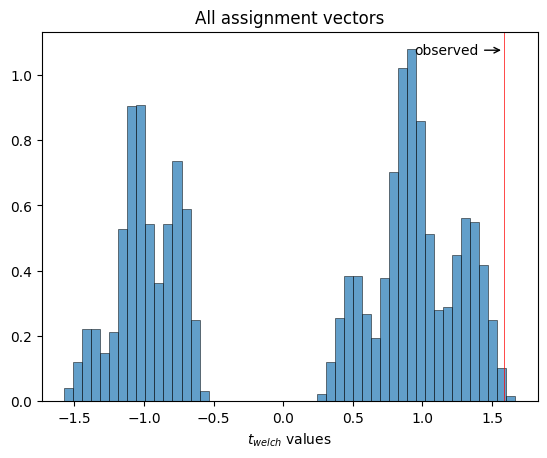
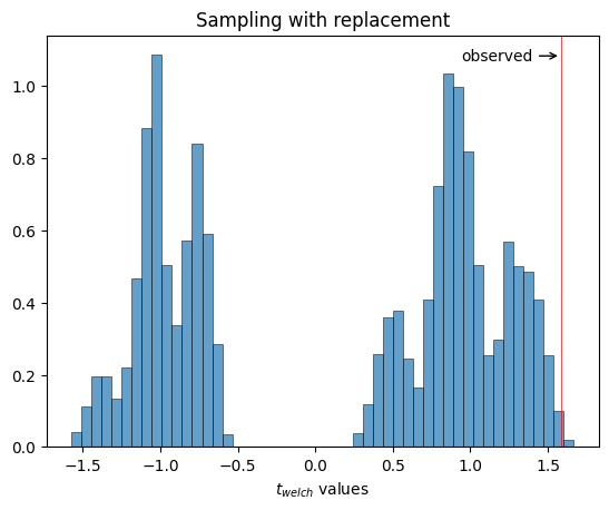
The p-values are similar (for this trial):

    exact p-value: 0.00185
estimated p-value: 0.00287

Since sampling with replacement creates duplicates for 12% of draws, there will be increased variance in the resulting estimate of the FEP. I ran 500 trials for both sampling with and without replacement, again using $k = N_\text{comb} / 4$. The plot below shows the numerator of the Fisher exact p-value. It’s the number of samples (including the observed) where the test statistics was >= the observed test statistic, for all 500 trials, for both sampling with and without replacement.

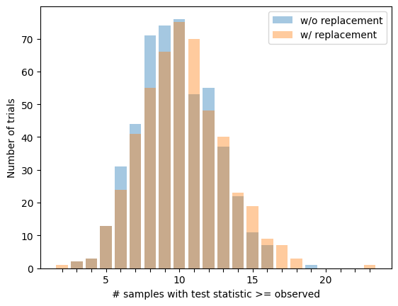
The distributions are very similar, but the variance is larger when sampling with replacement.

                 variance
w/o replacement: 6.667
 w/ replacement: 8.219

                 % increase
         in var: 23.3%
          in sd: 11.0%

Conclusion

Analyzing a Bernoulli trial as if completely randomized: common practice and totally fine

Sampling from all $n_{total}!$ permutations of the original assignment vector instead of the $N_\text{comb} = \binom{n_\text{total}}{n_\text{treat}}$ combinations of 1s and 0s:

• the difference is effectively to sample with replacement vs sample without
• when $k / N_\text{comb}$ is small, there is little to no difference
• when $k / N_\text{comb}$ is larger, sampling with replacement increases variance in p-value estimates

Whether the increased variance is an issue will depend on the application, of course. We should generally prefer the estimation method with lower variance, though, and this seems like a fairly easy change to make.