FRT & Interference: A General Method for Detection
Reference
Aronow, P. M. (2012). A general method for detecting interference between units in randomized experiments. Sociological Methods & Research, 41(1), 3–16.
Aronow’s paper proposes a specific Fisher Randomization Test (FRT) based on a known “distance” between units.
Two things I want to do:
- Replicate some of Aronow’s Simulation Studies
- Add a twist to the simulations by
- Allowing for “unlucky” fixed sets by randomly making some units “immune” to interference
- See if I can find a way to guard against these unlucky fixed sets
Replication
Aronow’s procedure
- Select an for rejecting the null hypothesis of no interference.
- Choose a random “fixed set” among the control set, with size . All statistics for the test are calculated within the fixed set.
- For each unit in the fixed set, calculate the distance to the nearest treated unit, .
- The baseline statistic, , is the absolute Spearman rank correlation between outcome and (both restricted to the fixed set).
- Calculate the same statistic across randomizations
- Randomize the treatment assignment for all units except the fixed set (shuffling 1’s and 0’s)
- For each unit of the fixed set, re-calculate the distance to the nearest treated unit,
- Calculate , the absolute Spearman rank correlation between the (fixed) and (new)
- Calculate and reject if
Aronow explains the use of the fixed set:
without further steps, randomization inference is capable of testing only the joint significance of both direct and indirect effects, rather than either individually.
A solution lies in developing a conditional permutation test for which the treatment status for a “fixed” subset of units remains invariant, so that the randomization inference is testing only the significance of indirect effects on this fixed subset.
For step 6, you could add 1 to both numerator and denominator of the -value (I did), but it shouldn’t make much difference for the simulations here.
Replication results
For the replication, I used fewer trials but the same number of randomizations per trial.
 |
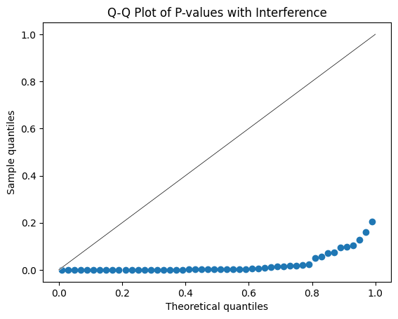 |
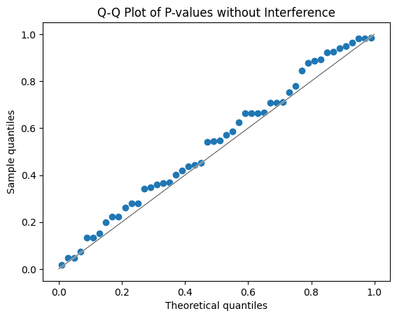
The plots above show results similar to Aronow’s Figure 1. However, for the trials with interference I got 90% rejection vs Aronow’s 83%. This is a big enough difference that it’s likely not due to chance. I have not been able to find the source of the discrepancy, but I’m reassured by the alignment of the main conclusions.
The plots below are also very similar to the top of Aronow’s Figure 2.
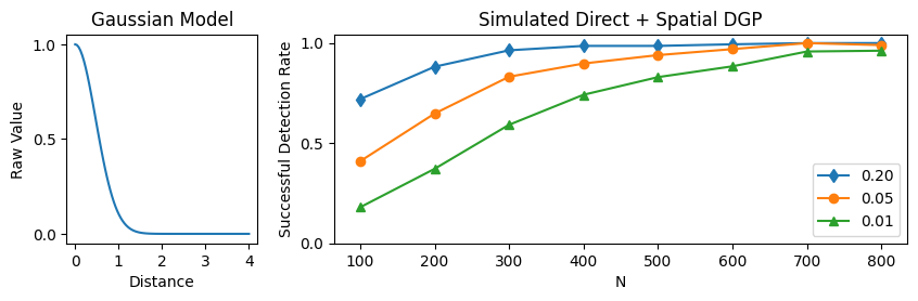
Right: Rejection rates for α = 0.05, 0.10, 0.20.
For my purposes, this is sufficient replication.
Lucky / unlucky fixed sets with the original DGP
Assuming distance-based interference, some fixed sets will produce stronger Spearman values ( close to 1) and some will produce weaker values ( close to zero). In other words, some random choices will produce fixed sets with stronger signals and some will produce weaker signals.
In Aronow’s Gaussian model, the outcome with interference is given by
So, there is a random component to the outcome , but the interference component is deterministic based on and distance.
Recall that is the rank correlation (within the fixed set) between and , where is the distance to the closest treated unit. I took 200 samples from the DGP (Gaussian model, 400 units, 200 control), and for each of those 200 samples I took 200 random fixed sets of 100 units each from the control units. I calculated for each of those fixed sets, for both the null (no interference) and with-interference simulations, and plotted the histograms.
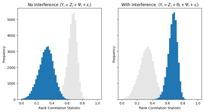
There’s some overlap, but there were no iterations with . Basically, this reflects what the QQ-plots above show: The null and with-interference cases are easily distinguishable. Put another way, the with-interference fixed sets will usually be “lucky”.
Adding “immunity” to the interference DGP
To degrade the inference signal, I removed some of the interference. I made some units “immune” to others’ influence while maintaining their influence on others, by setting some to zero.
Using the same settings as earlier, I added a large number of immune units, chosen randomly:
So 25%, 50%, or 75% of all units were randomly selected to be immune.
As expected, the rejection rate decreases:
            Rejection Rates
            with α = 0.05
  Original: 0.899
100 Immune: 0.626
200 Immune: 0.346
300 Immune: 0.131
The QQ-plot also gets closer to uniform:
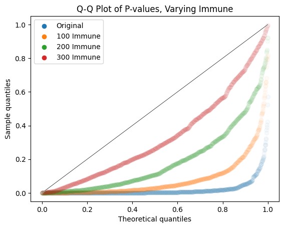
And the histogram of values approaches the histogram of the null DGP. The plot below repeats the histograms for above, but with 50% immunity (from receiving interference) in the with-interference DGP.
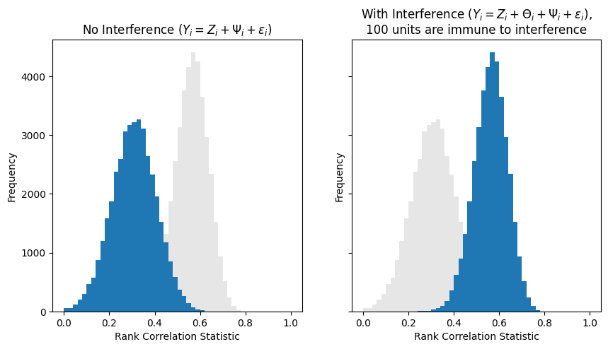
So, as intended, the added immunity weakens the interference signal overall, and will create more unlucky fixed sets. The interference is still present, though, and we want to find a robust way to detect it.
Guarding against unlucky fixed sets
What if you choose a subset with low signal? If you have some way of guessing which subsets have the clearest signal, you should use that, but if you don’t, how can you guard against an unlucky choice of subset?
Using multiple fixed sets
My initial idea was to choose multiple fixed sets, and then somehow combine the information from all of them. The more subsets you have, the more likely at least one of them has a strong signal.
The modified procedure, for getting raw -values from multiple subsets:
- Select an for rejecting the null hypothesis of no interference.
- Choose K random fixed sets among the control set, each with size . All statistics for the test are calculated within the fixed sets.
- Do the following separately for each fixed set. Compute one conditional ‑value per fixed set, treating each set as the fixed controls for its own conditional test.
- For each unit in the fixed set, calculate the distance to the nearest treated unit, .
- The baseline statistic, , is the absolute Spearman rank correlation between outcome and (both restricted to the fixed set).
- Calculate the same statistic across randomizations
- Randomize the treatment assignment for all units except the fixed set (shuffling 1’s and 0’s)
- For each unit of the fixed set, re-calculate the distance to the nearest treated unit,
- Calculate , the absolute Spearman rank correlation between the (fixed) and (new)
- Calculate
Combining -values
Rereading Aronow’s paper I saw that combining -values from multiple fixed sets was already partially covered:
the values for multiple subsets may be combined to obtain a single value for the entire sample (e.g., Kost and McDermott 2002) if a covariance matrix for the values is known
Unfortunately, I don’t know the covariance matrix for the values here, and I suspect there are many real-life situations where it would be hard to determine. What should we do?
MinP?
I initially tried the MinP procedure, with Aronow’s FRT in an inner loop and a permutation test in the outer loop. Essentially, MinP is a permutation test with Tippett’s method as the statistic (combine -values by just using the min). That turned out not to work; the rejection rate was worse than the single-fixed-set rejection rate and got worse as the number of fixed sets was increased. This might make sense because MinP is designed for sparse situations with one extremely strong -value among many nulls. In the current situation there’s likely some signal in all of the subsets.
MinP procedure but Fisher’s method?
Using the same FRT-within-permutation test, I replaced Tippett’s method with Fisher’s method: . In Fisher’s method, the -values should be from independent tests, and the combined -value has a distribution. Neither of those are necessary here, because the combined -value is just used as a statistic within the permutation test. (A bit more technical: The null distribution is generated through permutation. This is true for Tippett’s method as well. The -values should be independent, but in MinP the method is just used as a statistic.) This worked pretty well, and works increasingly better with more fixed sets.
Stouffer’s method?
I then tried the same procedure with Stouffer’s method. Stouffer’s method produces a -value instead of a -value, but again, we’re just using it as a statistic in the permutation. It’s less sensitive to extremely small -values than either Tippett’s or Fisher’s methods. Stouffer’s method seems to work slightly better than Fisher’s method.
Results
For simulations, I used
The values for , , and are all low. Even with these values, the simulations are very time consuming, and I’m ok with rough results here.
| # Fixed Sets | ||||
|---|---|---|---|---|
| Interference | Method | 3 | 5 | 10 |
| No | MinP | 0.032 | 0.024 | 0.018 |
| Fisher | 0.046 | 0.042 | 0.052 | |
| Stouffer | 0.046 | 0.042 | 0.050 | |
| Yes | MinP | 0.342 | 0.348 | 0.254 |
| Fisher | 0.480 | 0.546 | 0.592 | |
| Stouffer | 0.492 | 0.552 | 0.592 | |
The null DGP has roughly the correct rejection rate, but a little low for MinP with 5 and 10 subsets. For the DGP with interference (and 200 immune), recall the 1-fixed-set rejection rate was 0.346. MinP doesn’t improve the rejection rate with 3 or 5 fixed sets, and in fact does worse with 10 fixed sets. Fisher and Stouffer both improve the rejection rate, with Stouffer doing slightly better, and they get better with more fixed sets.
| # Fixed Sets | ||||
|---|---|---|---|---|
| Units Per Fixed Set | Method | 3 | 5 | 10 |
| 100 | MinP | 0.342 | 0.348 | 0.254 |
| Fisher | 0.480 | 0.546 | 0.592 | |
| Stouffer | 0.492 | 0.552 | 0.592 | |
| 75 | MinP | 0.352 | 0.350 | 0.266 |
| Fisher | 0.484 | 0.556 | 0.608 | |
| Stouffer | 0.490 | 0.558 | 0.630 | |
| 50 | MinP | 0.286 | 0.274 | 0.192 |
| Fisher | 0.428 | 0.482 | 0.572 | |
| Stouffer | 0.458 | 0.504 | 0.592 | |
To see if smaller fixed sets might work better (by improving the chance of a stronger signal), I reduced the fixed set size to 75 and 50.
- Having 75 units per fixed set seems to work slightly better, and MinP with 3 or 5 fixed sets gives slightly better than 1 fixed set without adjustment, but the differences are small and not statistically significant for typical values of .
- Having 50 units per fixed set seems to be worse for all three types of adjustment.
Something simpler?
The nested permutation test for the methods above is complicated and time consuming. It would be nice if there were a simpler, quicker method, but I haven’t found any. I tried multiple other metrics in place of Spearman’s , trying to find a metric that might be more robust to sparse signal in a single fixed set, but haven’t found anything that has worked yet.